Amazon Berkeley Objects

Amazon Berkeley Objects

Today, online commerce and product sales platforms have changed the way people buy and sell things. changed the way things are bought and sold. Companies such as Amazon and eBay have set a new standard, offering a huge variety of products worldwide. At In this context, it is important to be able to identify and categorise products quickly and accurately in order to to improve the user experience, manage inventories and strengthen marketing strategies. marketing strategies. Deep learning technologies and convolutional neural networks offer powerful tools to address these challenges. powerful tools to address these challenges. These technologies make it possible to analyse large amounts of product images and extract key features. Automating these processes not only saves a lot of work, but also improves the accuracy and consistency of product information, thereby of product information, which is important for making business decisions and satisfying customers. and customer satisfaction.

The Amazon Berkeley Objects (ABO) dataset is a very useful resource, as it provides detailed product images and data that can be used to train and evaluate models. detailed product images and data that can be used to train and evaluate deep learning models. deep learning models. With this data, advanced systems can be developed that not only recognise products and their features but also products and their features, but also suggest similar products, improve navigation and search in commerce navigation and search on e-commerce platforms, and personalise recommendations for users.

Dataset: Amazon Berkeley Objects

Aim

The main aim of this project is to develop a neural network that, based on product images, can identify and categorize product characteristics. This includes recognizing brand, color, type and other important specifications. To archive this objective, we must solve a rethink some things of the dataset. This dataset it is about 826.757 entries (fully merged with duplicated values still) and there are a lot of missing values across the possible labels

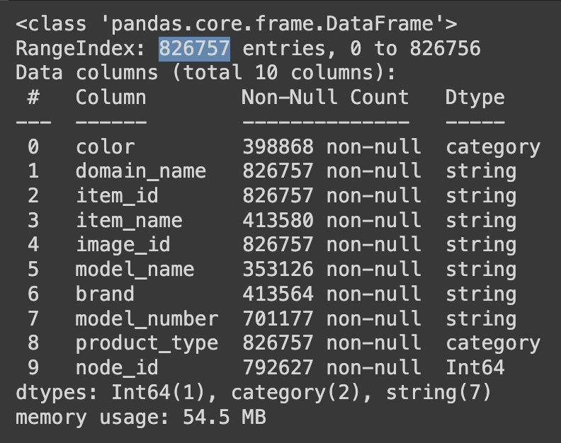
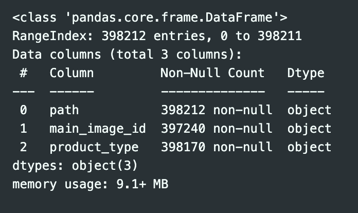
Here we can see that there are some great possible columns with almost no missing values, such as “prodcut_type” or “node_id” which has no (or almost) missing values. But others like color or brand will need more prepossessing to make them work in a neural network. Also, we have to keep in mind that the missing values they are not from the same row. For example, to highlight better the problem, suppose that the row number one of the dataset is a chair, number two a table and number three a desk. Peprahs it could happened that in row number one do not have any color assigned (missing value), but in number two and three they have, and row number two do not have brand, but it has all the others. The problem here is that if you want to predict three columns, we have to make three different preprocessing to the data to make it more accurate. Perhaps one of them is the class is not balanced and in other perhaps it is. So, in this article I decide to put focus in the process of just one label, which is “product_type”, but keep in mind that in the final solution I made this process to the other labels. Just not to make it very long

Metadata Dataset

This exploratory analysis aims to provide a detailed overview of the characteristics present in the product dataset. Each attribute is examined to highlight its potential importance in understanding and classifying product characteristics.

The datasets are divided in two:

• Structured data (Listings): This includes the Listings file and its metadata, which contains well-defined and organised information on product characteristics.

• Unstructured data: This includes the product images, whose information is less structured and requires additional processing to be used effectively.

• item_id (nominal): Unique identifier of the product.
• domain_name (nominal): Domain of the website where the product is sold. Identifies the sales platform and can be useful for data source analysis.
• item_name (nominal): Name of the product in different languages.
• 3dmodel_id (nominal): Identifier of the 3D model of the product.
• brand (nominal): Brand of the product in different languages. Important for brand identification.
• bullet_point (nominal): Product highlights or features in different languages. Provides product details that can be used for descriptions and feature analysis.
• colour (nominal): Colour of the product in different languages and standardised values. Important for the classification of products by colour.
• colour_code (nominal): Hexadecimal colour code of the product.
• country (nominal): Country where the product is located, in ISO 3166-1 code. It may be relevant for the analysis of geographical distribution and origin of the product.
• item_dimensions (numeric): Product dimensions (height, length, width) in inches. Important for the classification of products by size.
• item_weight (numeric): Product weight in pounds.
• main_image_id (nominal): Identifier of the main image of the product.
• marketplace (nominal): Platform for selling the product.
• material (nominal): Product material in different languages. Important for the classification of products by material.
• model_number (nominal): Model number of the product.
• node (nominal): Categories of the product within the category hierarchy. Important for product classification and organisation into hierarchical categories.
• other_image_id (nominal): Identifiers of other images of the product. Useful for additional views of the product.
• product_type (nominal): Product type. Important for the classification and organisation of products by type.
• spin_id (nominal): Identifier of the product in the inventory system.

Metadata of the Images-Small file: this file contains specific information about the images associated to the listed products.

• image_id (nominal): Unique identifier of the image, which refers to the main_image_id of the listings file.
• height (numeric): Height of the image in pixels.
• width (numeric): Width of the image in pixels.
• path (nominal): Path where the images are saved.

Not all of this data is gona be useful later.

Architecture

As this is one of my first projects on CNN, I consider a lot of possibilities and decided for one of them, there were a lot of things that make this decision: viability, difficulty and hardware was another one. Reminder that I made all this project locally, without any cloud.

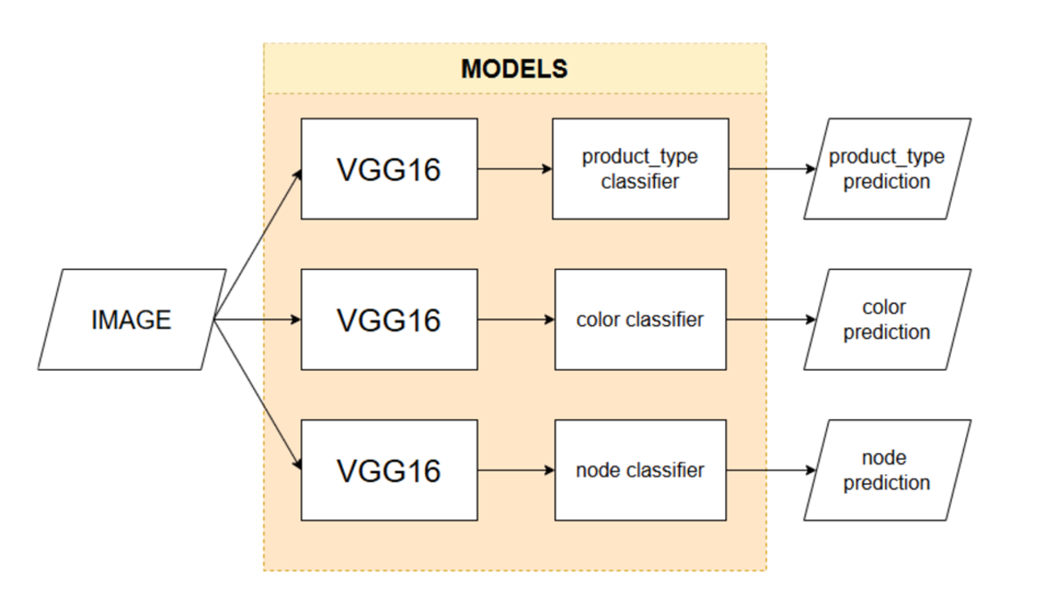
During data preprocessing, it was identified that processing each target variable differently provided an advantage, due to the raw data distributions. In order to optimize each class individually, it became necessary to create multiple models for classifying the data. This is because the specific training for each target variable must be independent, allowing for preprocessing that best fits each one.

The drawback of this approach is that a VGG16 model (others could have been used, but for reasons discussed later, VGG was chosen) is required for each value being predicted, leading to higher training costs. However, the clear advantage is that each model specializes in a single feature, which is particularly beneficial when performing fine-tuning, as there is no destructive interference between the data. Another benefit of this approach is the ability to use transfer learning with different models if one fits a specific variable better.

Alternative Architecture: B-CNN

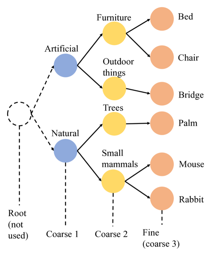
The B-CNN is a solution I considered implementing to maintain a hierarchical order between layers and improve the accuracy of predictions. The key idea is that the model would make predictions progressively, from broader categories to more specific ones. This approach can help reduce significant errors. For example, if the model has an accuracy of 70%, I would prefer it to make mistakes on the final, more specific categories, rather than at the broadest level. In other words, it’s better for the model to confuse a bed with a chair than with a mouse—a much larger mistake in terms of classification. The loss function in the B-CNN is designed to take into account the predictions at each layer, minimizing the chance of a major error by ensuring that predictions become progressively more precise as they pass through each layer.

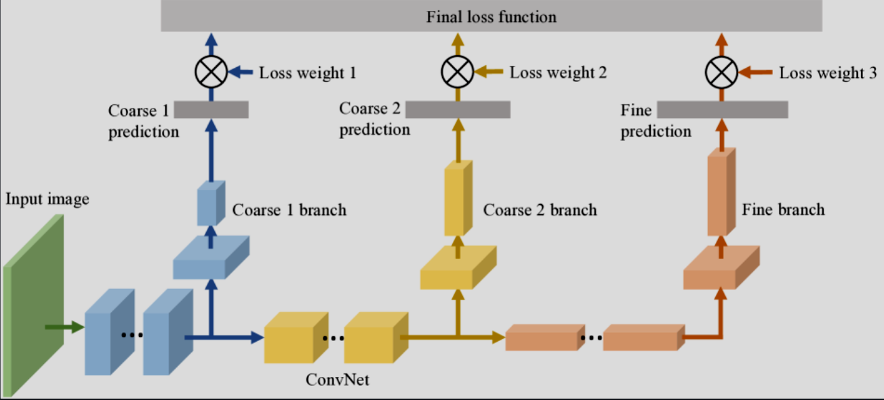
The idea is way more complex but here is the link where I got the idea: Article: B-CNN Article

In my case:

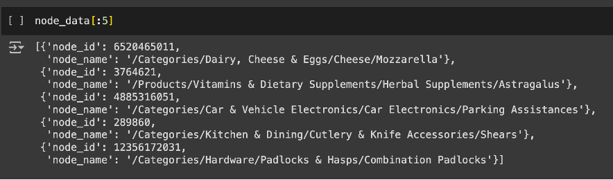
As it is seen, in my case is also divided in subcategories to make it every time more specific, that is the idea of the column, the reality is completely different, because they not have the same root, some of them there are in different languages, and they do not have the same de depth (as it seen). So this column has a lot of potential, but amazon did not make the best job of making this label useful (I explain it quite shortly but I spent hours and even days to make this work). But the solution was pretty original.

Preprocessing

In this case, we are going to put our focus in one label for preprocesisng (product_type), but in the real project I made three diffrent preprocesing for each label.

I did not include all the code here, only the more important and visual stuff

Merge of metadata

After identifying and eliminating irrelevant attributes, it was decided to unify the metadata of the files into a single dataset. This unification facilitates the analysis by consolidating all relevant features in one place, reducing the complexity of the modelling process and avoiding data integrity and redundancy issues. In addition, working with a single dataset is more computationally efficient and simplifies the identification and handling of missing values.

Missing values and duplicated data

After unifying the data, we identified and removed duplicate images to avoid redundancy and potential bias, and to optimize the efficiency of the training process. Duplicate images do not provide additional information and could skew the model’s predictions. Additionally, we assigned product attributes to both the main and secondary images. This ensures that each image contains complete and relevant information, enhancing the model’s ability to learn and make accurate predictions.

merged_df.info()

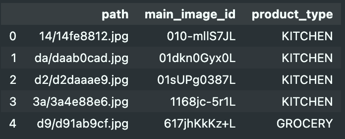
merged_df.head()

Label Preparation

Managing 512 unique product types with class imbalance posed a significant challenge. Training a neural network with so many classes often lead to the model overfitting to the most frequent ones, neglecting the minority classes.

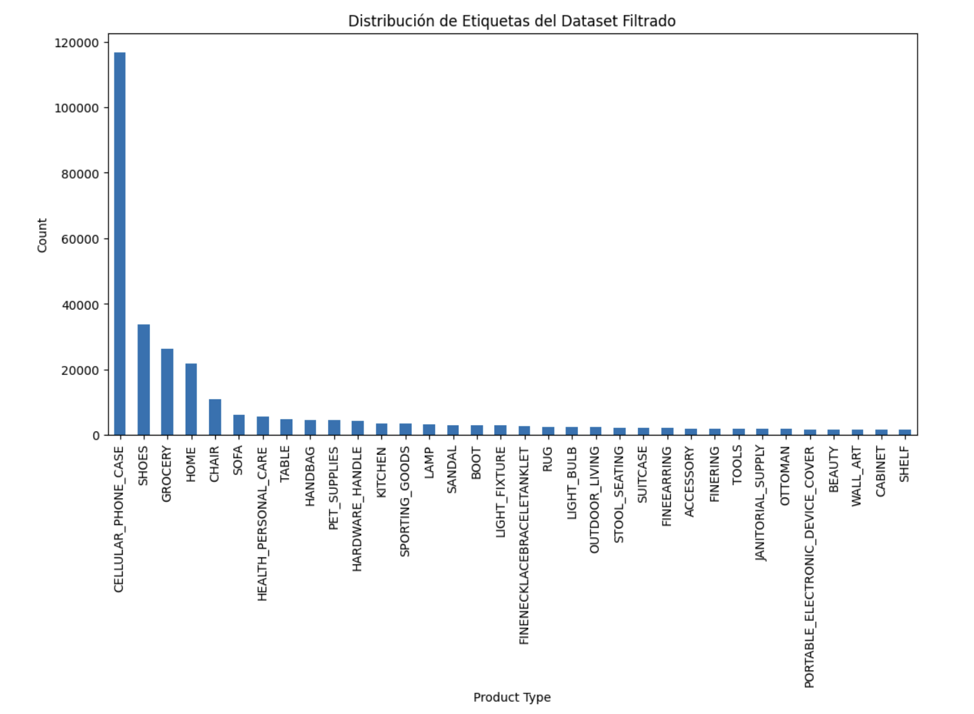
To mitigate this, we decided to cap the maximum number of photos per class at 2000. This threshold was chosen to reduce bias towards overrepresented classes while ensuring the model could still learn the necessary features for each class. It also helped keep the computational requirements within our hardware limits.

The second issue was the sheer number of product type categories—512 values in total—which was too large for our available resources. We prioritized the most meaningful categories, paying attention to how they were defined. Clear categories like “cell phone case” and “chair” were easy to work with, but others like “home” and “grocery” were too broad, including subcategories that overlapped with more specific labels (e.g., some armchairs were labeled as “home” while others were in “couch”). To address this, we removed overly general categories like “home” and merged similar ones, such as consolidating all types of footwear under “Boots,” “Shoes,” and “Sandal.”

Although we couldn’t solve all these issues perfectly due to time constraints, we implemented several strategies to improve model performance across seven iterations. Training was done on a local machine with an i7 12700k processor, 3060ti GPU, and 32GB DDR5 RAM. This setup significantly reduced training time compared to using Colab, but each iteration still took about 400 minutes. We typically left training running overnight, allowing us to spend the day adjusting the model and planning new iterations.

Model Iterations

In this chapter, I will explain the progress of the model and how I improved it over time. I’ll explore various possibilities that could enhance its accuracy. There were a total of seven iterations, in some of them showing gradual improvements, with one iteration yielding the best results so far. However, there is still room for further optimization and refinement.

Iteration V1 VGG16

The first iteration counted with 42 possible values for the label with 2000 photos each, VGG16 was the first pretrained model that was used modifying some hyperparameters such as the optimizer (Adam) and the loss algorithm. And from the first iteration I applied progressive fine tuning, the first 20 epochs the layers are frozen (so the weights of the hidden layers are not modified and just the dense layers are adjusting) with a learning rate of 0.01. And after those epochs the last 20 layers are unfrozen. As for the image input, the ABO dataset documentation mentions that it has a maximum 256px, but after some iterations it was observed in more detail that most of the images did not have 256x256 of the images did not have 256x256 dimensions. For that reason, we considered using using VGG16 with 224x224 entries.

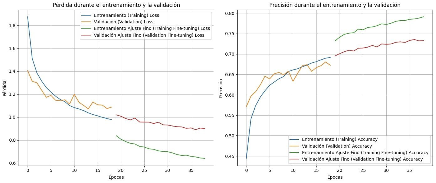
Loss in validation: 1.2007800340652466

Validation accuracy: 0.6813859939575195

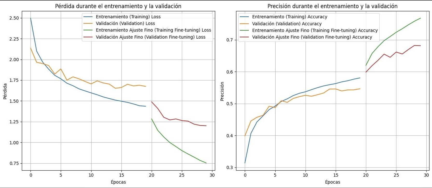
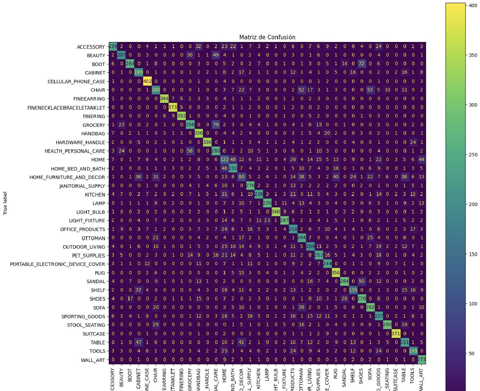
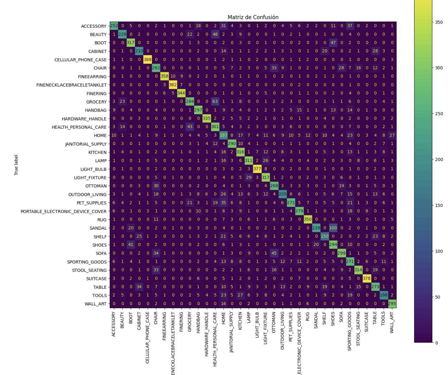
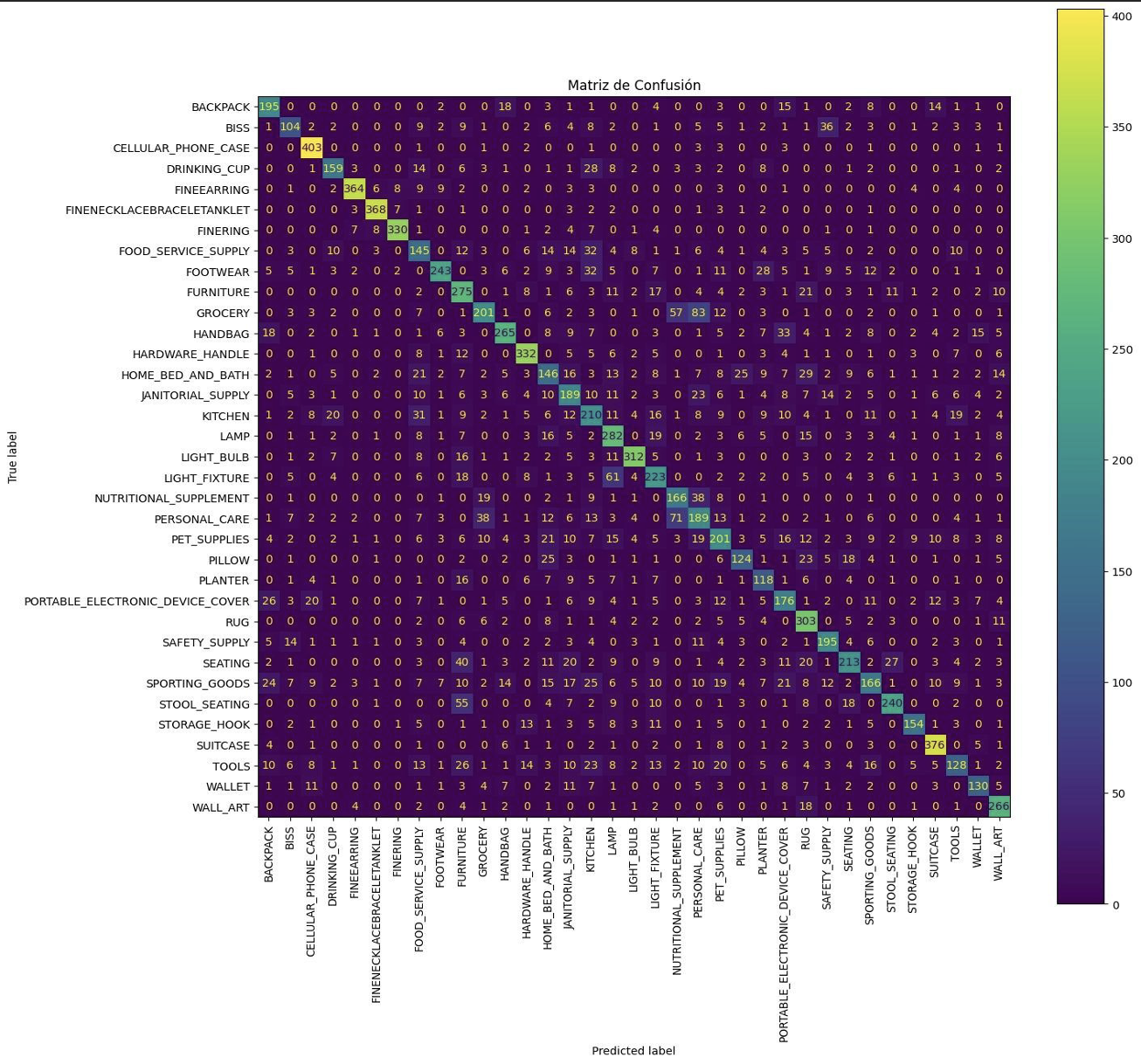
The results of the first iteration were promising, achieving nearly 70% accuracy on a dataset with 42 possible labels. Based on the training graphs, it’s clear that additional epochs could have further improved performance. The confusion matrix also highlighted some issues, such as the presence of broad categories, which I had previously mentioned. For the next iteration, I addressed some of these challenges to refine the model’s performance.

Iteration V2 VGG16

In the second iteration, progressive fine-tuning was adjusted, and optimizers along with callbacks were added. The most important callbacks were early stopping and model checkpoints, which significantly increased the efficiency of the training process.

Another extremely important feature introduced at this stage was data augmentation, which included the following techniques:

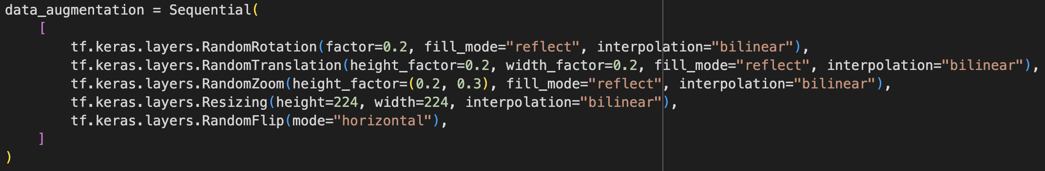
With the following results:

Loss in validation: 0.899906396865844

Validation accuracy: 0.7329152822494507

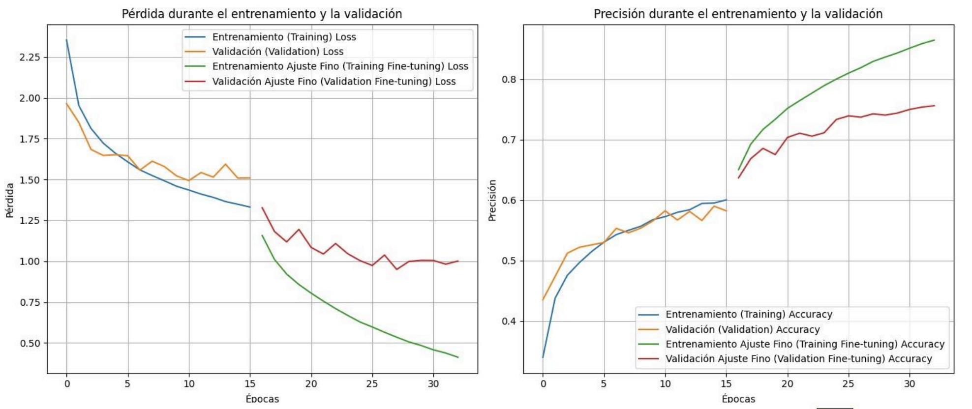
As can be seen the progressive fine tuning was very beneficial in terms of model accuracy, but overfitting can also be observed in the latter part of that training at the time of unfreezing the layers, perhaps a rather high overfitting was allowed, causing each epoch that passed the loss and accuracy to separate between training and validation. Despite having that overfitting, the validation loss continued to drop for each epoch so it’s not all bad.

Iteration V3 ResNet50

In this case no metrics were achieved, a new pre-trained architecture such as ResNet was used to meet the needs of the photo input (256 x 256) without the architecture such as ResNet was used to meet the needs of the photo input (256 x 256) without progressive fine tuning. progressive fine tuning. As mentioned above, this iteration can be considered as a failure since after 30 epochs failure since after 30 epochs (and a very slow training due to the photo input) the accuracy stagnated at 29%. accuracy stagnated at 29%. This is why it was decided to interrupt the training and to change the architecture again, also correcting architecture again, also correcting some aspects of the labels, and looking for improvements in the preprocessing of the improvements in image preprocessing.

Iteration V4 InceptionV3

For this new iteration, a slightly faster and more efficient pre-trained model was considered in terms of training, since with ResNet too much time was wasted on what we considered not profitable. ResNet, as investigated, is very deep and contains residual blocks to skip connections, which can lead to more robust results. Beyond the fact that Inception V3 has a very complex architecture, it is designed to optimize computational resources (something that was needed). As mentioned, the images were rescaled to 299 x 299 to meet the needs of the model.

• Loss in validation: 0.8999063968658447

• Validation accuracy: 0.7329152822494507

As can be seen, again there is an overfitting in the model, something that until now we had tried to mitigate by data augmentation, but from here on alternatives were sought to solve this problem that were affecting the performance for many iterations. And of course, I kept making corrections to the tag, making merge, eliminating unnecessary ones or even adding some speculating that it could be a good option. Despite all these problems, and rescaling the image with “noise”, the accuracy was good.

Iteration V5 VGG16

In this new iteration, it was decided to go back to VGG since there had been a great accuracy with this model but without adding all these new settings, with potential to further increase the accuracy of the V2 iteration. In this case, it was decided to use VGG16 with 256 x 256 pixels, and to mitigate the overfitting an L2 regularization was used. L2 is a technique to add a penalty to the high weights of the model, that way you can generalize more to unseen data and solve the dragging problem. In addition to that, it was decided to eliminate the progressive fine tuning in order to find from the first epoch the fine tuning since we had this new method to reduce overfitting (also because this new strategy had never been tried before). It was left for one night training, expecting a great result the next day, but again it was a failure since after 50 epochs it had reached only 43% without improvement. That is why the training was cancelled to try to find new ways. Then, analyzing in more detail the progression of the model during those epochs, it was observed that it could have been some issue related to the learning rate, since both loss and accuracy were improving very slowly for about 40 epochs.

Iteration V6 VGG16

Due to time constraints, this was going to be the last iteration to be performed, so we tried to optimize as much as possible what had given results previously. Therefore, VGG16 was used, but this time using 100% of the images, i.e. 256x256. Some small adjustments were made to the label, we returned to the progressive learning rate that had given us very good results while trying to mitigate the overfitting with another less invasive technique. A dropout function (at 0.3) given by keras was used, this function has the objective of deactivating some neurons randomly, to generalize the data and avoid the network becoming dependent on specific neurons. The progressive fine tuning was divided in two stages as mentioned before, 25 the first phase with frozen weights and then another phase with 25 epochs unfreezing the last 20 layers (adam and the same learning rate as in previous cases were used).

• Loss in validation: 1.32392418384552

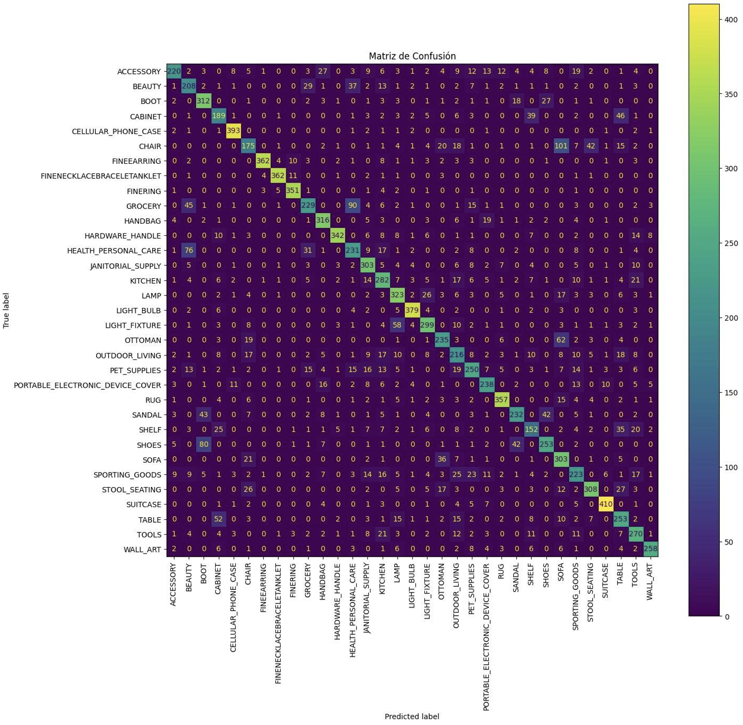
• Validation accuracy: 0.6500535607337952

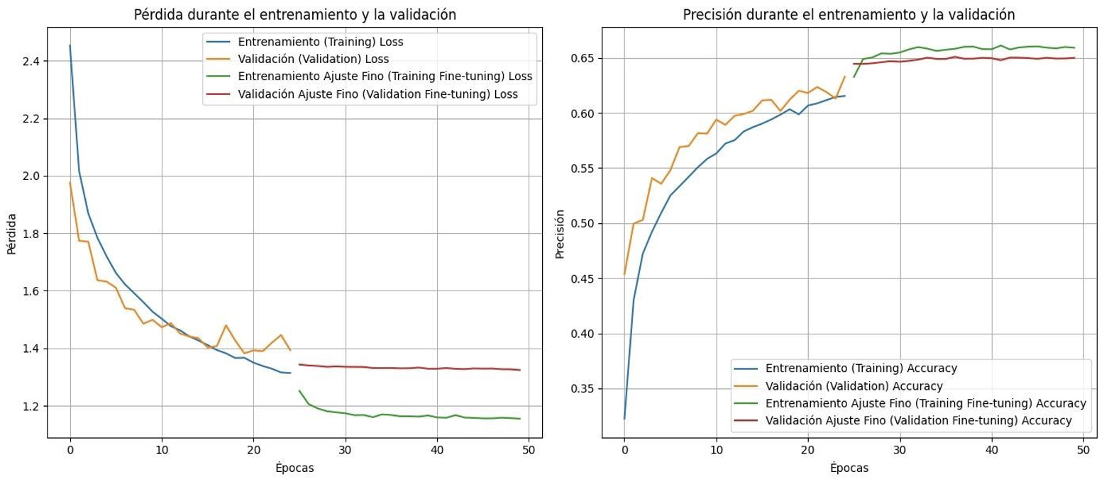
This model was the last one we had time to work on, and it is considered quite decent, we were able to fix the overfitting issue that kept me entertained for so many iterations, but in return, the overall accuracy did not end up so high (65%). The whole iteration design is a constant trade off, which is not easy to balance. Solutions related to iterations have been sought, although not specifically on accuracy (as more iterations and computational capacity will be needed). However, issues such as overfitting, labels and preprocessing, among others, have been addressed. To conclude this model, it is worth noting that there is still much to learn about both the world of computer vision and the data. With more knowledge, some of the paths of this model could be shortened or even further improved. However, the process of learning and testing the model was very time consuming, as models like the last one took between 6 and 8 hours (perhaps with more experience it would not take so long). If accuracy is to be improved, it is crucial to focus on the label. Some possible solutions include reorganizing or merging certain tags, or even eliminating several of them to simplify the dataset. These actions can help to obtain better model performance and fix current inconsistencies.

Conclusion

The study conducted on the Amazon Berkeley Objects (ABO) dataset demonstrated the challenges and potential of using deep learning techniques for product classification. Through iterative improvements and experimentation with different Convolutional Neural Network (CNN) architectures such as VGG16 and ResNet50, valuable insights were gained regarding model performance and dataset handling.

Key findings include the importance of preprocessing to address missing and duplicated values, especially in a dataset as large and diverse as ABO. Class imbalance also posed a significant challenge, which was mitigated by capping the number of images per class and consolidating similar categories. This approach helped prevent the model from overfitting to dominant classes while improving generalization for underrepresented ones.

The use of progressive fine-tuning, data augmentation, and callbacks like early stopping proved to be highly effective in improving model accuracy, with the best-performing iteration reaching over 73% accuracy. However, overfitting remained an issue, indicating the need for further regularization techniques or more balanced training strategies.

Further improvements could be made by refining the label hierarchy, exploring other model architectures, using some object detection model, and possibly leveraging cloud computing resources to handle larger-scale data and longer training times more efficiently.

Here is a video for Demo with the V2 iteration

Here is the notebook of the V2 iteration.

https://drive.google.com/file/d/1EjAnTSAilT7ZBMa9Izb3IaRqN7fAeIJJ/view?usp=sharing