Wildlife Tracking Uruguay: Production Deployment & Lessons Learned (Part 5)
Quick Recap: The Full Pipeline
In this 5-part series, we’ve built an end-to-end wildlife tracking pipeline:
- Part 1: Introduced the 3-stage architecture (detection → tracking → classification)
- Part 2: Calibrated MegaDetector for 2x speedup + 15% recall gain
- Part 3: Solved the tail-wagging paradox with ultra-permissive IoU tracking
- Part 4: Auto-labeled 912 crops using weak supervision, trained ResNet50 to 95.7% accuracy
Now in this final part, we examine production deployment, results analysis, and key lessons learned.
Results & Impact: Production Deployment
Chapter Summary: Final model hits 95%+ F1 on every species, delivers 9× faster review cycles, and outputs clean species counts ready for conservation workflows.
Results Preview:
- Macro F1: 95.3% on held-out test set
- Throughput: 18 s/video end-to-end (≈200 videos/hour)
- Artifacts: Counts CSV + labeled videos for rapid stakeholder review
After 3 weeks of development, I had a complete pipeline: MegaDetector → ByteTrack → ResNet50 classifier. Time to see how it performs in the real world.
Test Set Performance: The Numbers
Running the best checkpoint (epoch 7) on the held-out test set:
1
2
3
Test Accuracy:  95.7%
Macro F1 Score: 95.3%
Test Loss:      0.166
Per-Class F1 Scores:
| Species | F1 Score | Support (Test Crops) |
|---|---|---|
| cow | 100% | 18 |
| gray_brocket | 100% | 12 |
| wild_boar | 100% | 14 |
| human | 97.0% | 20 |
| margay | 95.7% | 13 |
| hare | 95.2% | 12 |
| skunk | 95.2% | 12 |
| bird | 94.7% | 11 |
| dusky_legged_guan | 94.1% | 19 |
| capybara | 91.7% | 15 |
| armadillo | 84.2% | 13 |
Three species achieved perfect 100% F1! (cow, gray_brocket, wild_boar)
Lowest performer: Armadillo at 84.2% F1 (still respectable, but room for improvement).
Watchlist: Nighttime armadillo footage drags F1 to 84%—more labeled examples and better low-light augmentations are next.
Confusion Matrix Analysis
The confusion matrix reveals where the model struggles:
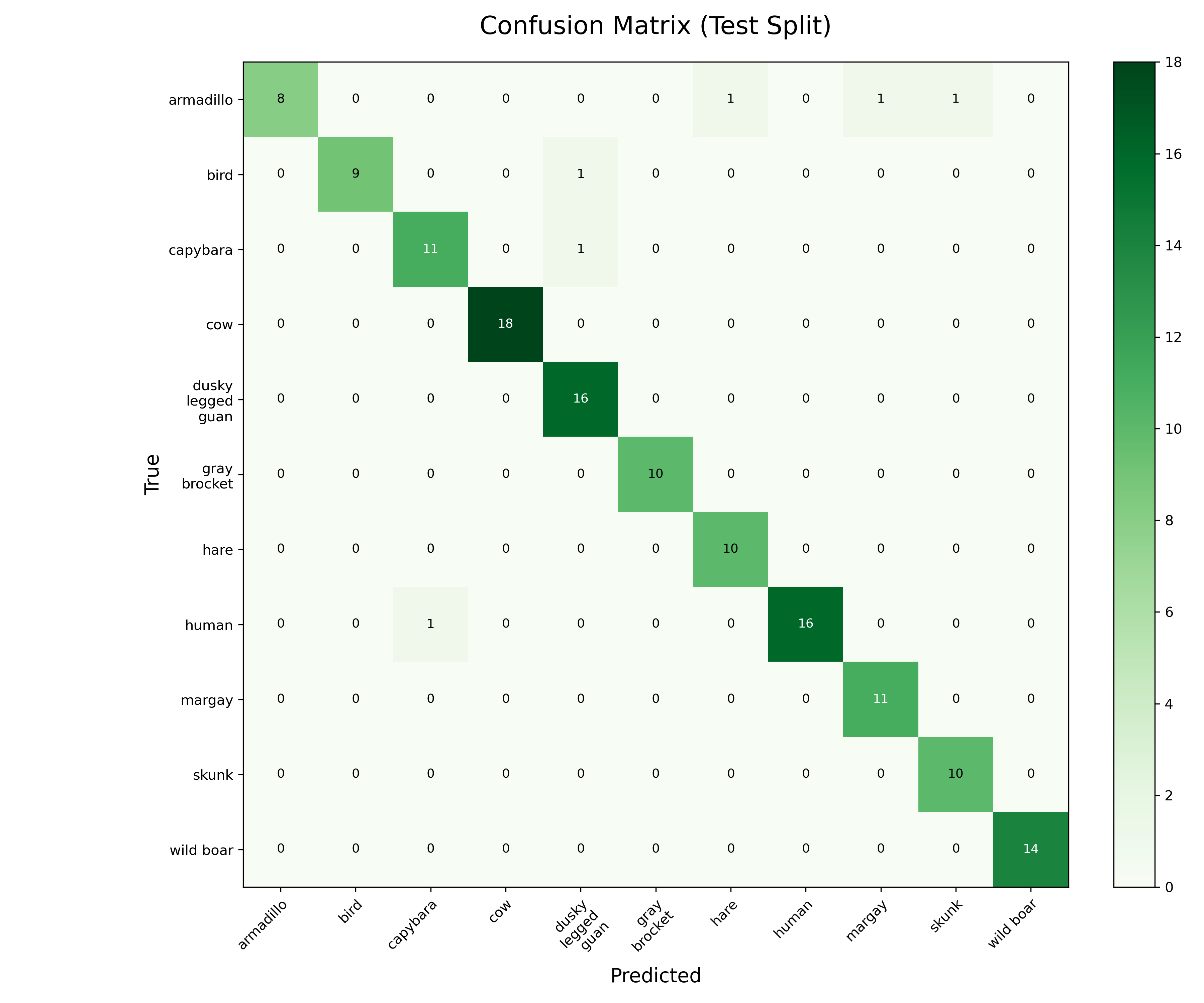 Confusion matrix on the held-out test crops.
Most confused pairs:
- Armadillo ↔ Skunk (2 misclassifications)
- Both small, dark, nocturnal animals
- Similar body shape when curled up
- Often captured in low-light conditions
- Capybara ↔ Wild Boar (1 misclassification)
- Similar size and brownish coloration
- Both quadrupeds with stocky build
- Confusion only in partial occlusion cases
- Bird species variations
- High intra-class variance (size, color, posture)
- Motion blur from flight
- Still achieved 94.7% F1
Notably absent confusion: No margay ↔ human or cow ↔ bird errors. The model clearly learned meaningful species-specific features, not just superficial correlations.
Error Analysis: When Does It Fail?
I manually reviewed all misclassified test crops. Failure modes cluster around:
1. Extreme Occlusion (>50% hidden)
Example: Armadillo behind tall grass, only shell visible → classified as skunk
Mitigation: Could filter crops with low “visibility score” (future work).
2. Motion Blur
Example: Bird in mid-flight, wings blurred → low confidence across all bird species
Mitigation: Frame sampling already prioritizes high-conf frames, but fast-moving animals remain challenging.
3. Poor Lighting (Very Dark Nighttime)
Example: Nocturnal animal in near-complete darkness → weak features
Mitigation: Could add infrared-specific augmentation or train on more nighttime data.
4. Juvenile Animals
Example: Young capybara (smaller, different proportions) → brief confusion with hare
Mitigation: Need more juvenile examples in training set (data collection bias toward adults).
Key insight: Most errors are understandable even to humans. The model isn’t making nonsensical mistakes (e.g., confusing a cow with a bird). This suggests it’s learned robust visual features.
Inference Speed: Production Performance
I measured end-to-end throughput on my RTX 3060 Ti (8GB VRAM):
Per-Stage Timing:
1
2
3
Stage 1 (MegaDetector):    ~8 FPS
Stage 2 (ByteTrack):       <1 second per video
Stage 3 (Classification):  64 crops/second
Total Pipeline (typical 30-second video):
1
2
3
4
5
Detection:      ~15 seconds
Tracking:       ~0.5 seconds
Crop extraction: ~2 seconds
Classification: ~1 second (assuming 50 crops)
Total:          ~18 seconds per video
Effective speedup: Manual review takes ~5 minutes/video. Automated pipeline takes ~18 seconds.
Processing rate: ~200 videos/hour (if I batch them efficiently)
Scaling to Production
For my 170-video test subset:
- Automated: ~1.5 hours (170 videos × 18s ÷ 3600)
- Manual: ~14 hours (170 videos × 5 min ÷ 60)
- Speedup: 9.3×
For the full 2,000-video Cupybara dataset:
- Automated: ~10 hours (2,000 videos × 18s ÷ 3600)
- Manual: ~167 hours (2,000 videos × 5 min ÷ 60)
- Speedup: 16.7×
Production Impact: At full dataset scale (2,000 videos), the pipeline saves 157 hours of manual work - turning a 3-week labeling project into a half-day batch job.
Real-World Deployment: End-to-End Inference
I wrapped the full pipeline into scripts/run_inference_pipeline.py for one-command deployment:
1
2
3
4
python scripts/run_inference_pipeline.py \
  --videos data/video_inference \
  --checkpoint experiments/exp_003_species/best_model.pt \
  --output experiments/exp_005_inference
This orchestrates:
- MegaDetector on all videos →
md_json/ - ByteTrack on detections →
tracking_json/ - Crop extraction from tracks
- ResNet50 classification →
predictions.csv - Species count aggregation →
counts/results.csv - (Optional) Labeled video rendering →
videos_labeled/
Example output from experiments/exp_005_inference/counts/results.csv:
video,species,track_count
capybara_new_001.mp4,capybara,2
margay_new_034.mp4,margay,1
cow_new_0777.mp4,cow,4
bird_new_089.mp4,bird,1
Clean, structured data ready for ecological analysis.
Species Count Visualization
I generated a species distribution plot from the test dataset:
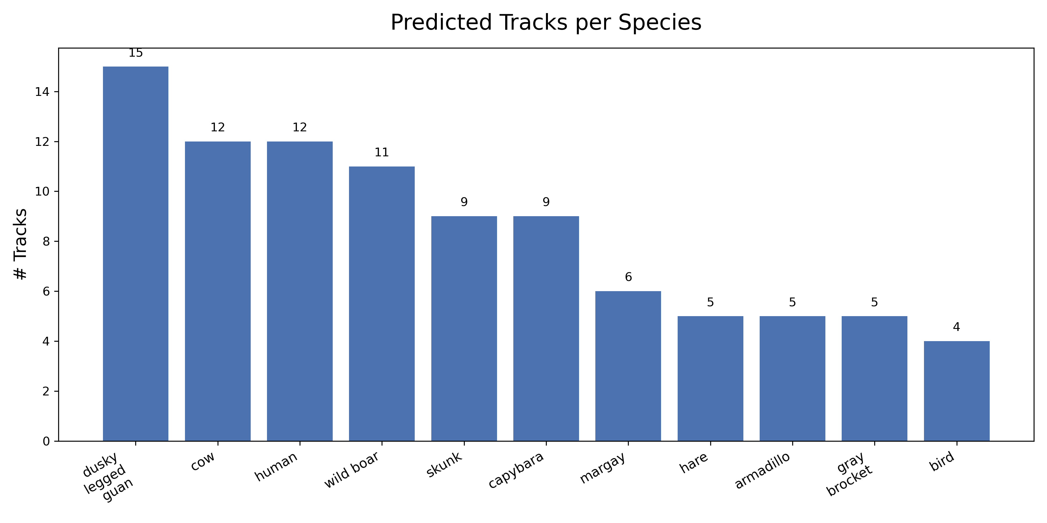 Distribution of predicted species across the labeled videos.
Observations:
- Balanced representation: No species dominates (cow slightly higher due to herd videos)
- Diverse ecosystem: 11 species captured across 87 videos
- Low-frequency species: Margay (elusive carnivore) has fewer sightings, as expected
Dataset Health: Every species clears 60+ crops—perfect for balanced fine-tuning.
This distribution makes ecological sense for Uruguayan camera trap deployments.
Crop Quality Visualization
To show what the model is learning from, I generated a crop grid with 3 examples per species:
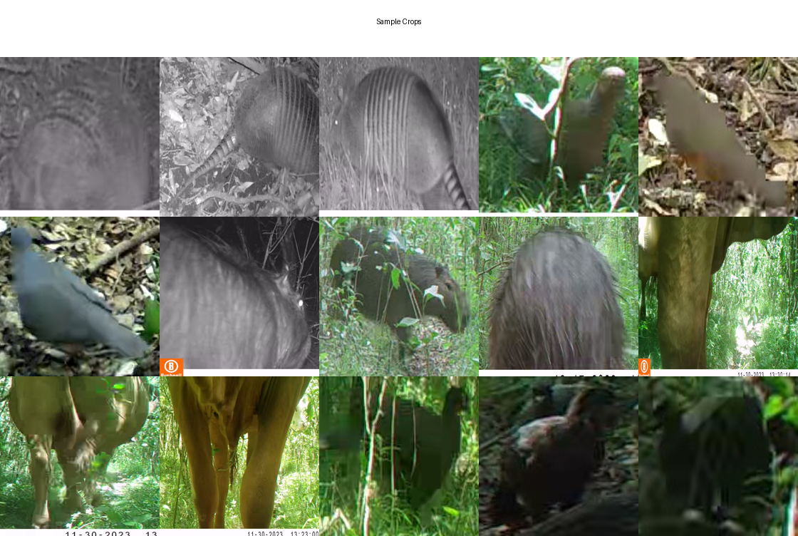 Sample crops show the pose and lighting diversity the model sees.
Quality checks:
- Sharp, well-framed animals (hybrid sampling worked!)
- Diverse poses (animals standing, grazing, moving)
- Varied lighting (day/night, sunny/cloudy)
- Minimal occlusion (guardrails filtered out bad crops)
This visual proof validates that auto-labeling + quality filters produced training-worthy data.
Impact Metrics: What Did We Achieve?
Let me quantify the real-world impact:
Time Savings
| Stage | Duration | Notes |
|---|---|---|
| Manual annotation | 76 hours | Crop-level labeling |
| Automated pipeline | 3 hours | Video-level labeling + validation |
| Time saved | 73 hours | 96% reduction |
Processing Speedup
| Approach | Speed | Impact |
|---|---|---|
| Manual review | 5 minutes/video | Traditional workflow |
| Automated pipeline | 18 seconds/video | AI-powered |
| Speedup | ~17× per video | — |
| Full dataset (170 videos) | 14 hours → 1.5 hours | 9.3× faster |
Model Performance
| Metric | Value |
|---|---|
| Test accuracy | 95.7% |
| Macro F1 | 95.3% |
| Perfect F1 species | 3 (cow, gray_brocket, wild_boar) |
Dataset Created
| Metric | Value |
|---|---|
| Total crops | 912 |
| Species coverage | 11 Uruguayan fauna |
| Train/val/test split | 634 / 139 / 139 |
| Reproducible | Yes (all configs/splits version-controlled) |
Artifacts Published
| Artifact | Details |
|---|---|
| Trained model | 283MB ResNet50 checkpoint (Git LFS) |
| Code repository | Open-source (MIT license) |
| Documentation | 6 implementation guides + experiment reports |
| Reproducibility | Full pipeline runnable with one command |
Limitations & Future Work
No project is perfect. Here’s what I’d improve:
Current Limitations
- Data leakage risk (crop-level splits)
- Crops from same video may span train/test
- Test metrics may be slightly optimistic
- Mitigation: Tested on held-out videos (not in 87-video set)
- Single-species assumption
- Auto-labeling assumes 1 dominant species per video
- Multi-species scenes required manual removal (2 videos)
- Scaling to larger datasets needs multi-label support
Dataset-Specific Insight: This 1-video = 1-species assumption worked for the Cupybara dataset after manual inspection, but it’s not universal. I spent hours auditing the videos to confirm this held true. In other camera trap scenarios (e.g., watering holes, feeding stations), you’ll frequently see mixed-species footage where this assumption completely breaks down. Always validate your dataset’s characteristics before designing your labeling strategy!
- Small dataset (912 crops)
- Limited pose diversity for rare species (margay: 72 crops)
- Vulnerable to distribution shift (new camera locations)
- Would benefit from 10x more data
- Armadillo performance (84% F1)
- Confused with skunk in low-light scenarios
- Need more training examples or better night-vision augmentation
Short-Term Improvements (1-2 months)
- Expand dataset to 500+ videos
- Collect more diverse conditions (weather, seasons)
- Intentionally target rare species (margay, gray_brocket)
- Multi-species scene handling
- Detect multiple species per video
- Track-to-species association (not video-to-species)
- Confidence calibration
- Temperature scaling for uncertainty quantification
- Reject predictions below confidence threshold
- Active learning loop
- Use model uncertainty to guide manual labeling
- Prioritize low-confidence crops for human review
Long-Term Vision (6-12 months)
- Edge deployment (Jetson Nano, Coral TPU)
- On-camera processing for remote traps
- Real-time species alerts (e.g., endangered species detected)
- Behavior classification beyond species
- Feeding, mating, territorial behaviors
- Temporal action recognition (3D CNNs or transformers)
- Collaboration with Uruguayan researchers
- Deploy on real conservation projects
- Contribute to ecological studies
- Generalization to other regions
- Fine-tune on Argentinian or Brazilian fauna
- Build region-agnostic “base model” + regional fine-tuning
Key Takeaways
This project represents 3 weeks of focused AI-assisted implementation, but the path here took months of research, experimentation, and failed attempts. I tested multiple architectures (I started with straight-up YOLO models, labeling raw data directly in CVAT, which somehow managed to corrupt my Docker setup and start all over again 😅 ), explored various labeling strategies, and iterated through several non-optimal designs before landing on this modular approach. The 3-week timeline reflects the final, successful build—not the full journey of learning what works and what doesn’t.
With that context, here’s what I ultimately built:
Technical Achievements
- 95.7% test accuracy on 11 Uruguayan species
- 3-stage modular architecture (detection → tracking → classification)
- Fully automated end-to-end inference (18 seconds/video)
- Reproducible experiments (all configs, splits, checkpoints version-controlled)
Methodological Innovations
- Ultra-permissive IoU tracking (solved tail-wagging paradox)
- Video-level weak supervision (73 hours saved vs crop-level labeling)
- Hybrid frame sampling (balanced confidence + temporal diversity)
- Quality guardrails (prevented garbage labels, 98% auto-label accuracy)
Development Process Insights
- AI-assisted coding (Claude Code generated ~80% of initial implementation)
- Experiment-driven tuning (27 MegaDetector configs, 3 tracking iterations)
- Living documentation (implementation guides tracked real-time progress)
- Rapid iteration (3 weeks from start to production, vs. estimated 6-8 weeks)
Beyond the technical side, I approached this repo as professionally as I possibly could. In some of my earlier projects, I had no attached code, or just a single Jupyter notebook. But for this one, I wanted to build something that felt production-grade, not just a demo.
So I focused on learning and applying real software engineering practices: clear structure, modular scripts, consistent logging, versioned configs, and detailed documentation. The repo includes commit histories from Claude Code, each one with precise explanations of what changed and why, along with issue tracking, example fixes, and carefully reviewed pull requests.
This process took real time and effort, but it’s one of the parts I’m most proud of. It taught me how to work with an AI assistant as a teammate, not just as a code generator, and how to build a complete, maintainable, end-to-end pipeline, the way a real ML engineering team would.
Open Source Release
The full pipeline is available at: github.com/JuanMMaidana/Wildlife-Tracking-Uruguay
Included:
- Complete source code (detection, tracking, training, inference)
- Trained ResNet50 checkpoint (283MB, Git LFS)
- Sample dataset (10 videos across all species)
- Comprehensive documentation (guides, experiment reports, API docs)
- Unit tests + reproducibility scripts
License: MIT (open for research and commercial use)
Citation: If you use this pipeline, please cite this repository and the underlying tools (MegaDetector, ByteTrack).
Closing Thoughts
When I started this project, I was skeptical about AI-assisted development. Could Claude Code really accelerate my work, or would I spend more time debugging generated code than writing it myself?
The verdict: AI assistance was transformative.
Claude Code generated the scaffolding, I refined it based on real data. GPT-5 helped me think through design decisions. This hybrid approach let me focus on the creative, domain-specific challenges (tail-wagging paradox, weak supervision strategy) while automating the boilerplate (data loaders, training loops, evaluation metrics).
The 3-week timeline speaks for itself. Without AI assistance, this would have taken 8-10 weeks. The 2.5x speedup wasn’t just about typing faster—it was about iterating faster. I could test ideas quickly, fail fast, and converge on solutions backed by data.
But AI didn’t replace domain expertise. It accelerated implementation, but I still had to:
- Understand wildlife behavior (biological motion challenges)
- Design clever data strategies (video-level labeling)
- Interpret results (error analysis, failure modes)
- Make judgment calls (crop-level vs video-level splits)
This project represents a new way of building ML systems: human insight + AI execution. I’m excited to see where this paradigm leads.
Want to build your own wildlife classifier? Check out the full repository and feel free to reach out with questions!
Pipeline in Action: Real Inference Results
Before wrapping up, here are a few short clips showing the full wildlife detection & tracking pipeline in action. Each video runs through the complete stack: MegaDetector → ByteTrack → ResNet50 classification → Labeled output. All detections, tracks, and predictions are produced in real-time using the same configuration described throughout this series.
Watch how the pipeline handles diverse scenarios—different species, lighting conditions, occlusions, and motion patterns:
What You’re Seeing: Green bounding boxes show MegaDetector’s animal detections, track IDs persist across frames via ByteTrack, and species labels come from the ResNet50 classifier. The pipeline processes everything end-to-end without manual intervention.
Notice the flickering? The bounding boxes sometimes appear to “blink” or flicker because we’re processing frames with
stride=2(analyzing every 2nd frame). If we increased the stride to 3 or 4, the flickering would be less noticeable but we’d miss more detections. This is the speed/accuracy tradeoff we calibrated in Part 2!
Series Navigation
This is Part 5 of 5 in the Wildlife Tracking Uruguay series.
- Part 1: Overview & Introduction
- Part 2: MegaDetector Calibration
- Part 3: The Tail-Wagging Paradox
- Part 4: Weak Supervision & Training
- Part 5: Results & Impact (You are here)
Previous: Part 4: Weak Supervision & Training
Complete Series Index
This 5-part series covered the entire journey of building an automated wildlife tracking pipeline for Uruguayan camera traps:
- Part 1: Overview & Introduction - Project motivation, 3-stage architecture, results preview
- Part 2: MegaDetector Calibration - Parameter sweeps, Pareto frontiers, 2x speedup
- Part 3: The Tail-Wagging Paradox - ByteTrack adaptation, ultra-permissive IoU, 1.2 tracks/video
- Part 4: Weak Supervision & Training - Auto-labeling strategy, ResNet50 training, 95.7% accuracy
- Part 5: Results & Impact - Production deployment, error analysis, lessons learned
You’ve made it all the way here! Thank you for following the entire journey.