Wine - Predicting Class

Wine - Predicting Class

This is a wine dataset donated in 1991 with the purpose of testing some IA tools, it has the objective of determinate the origin of the wines using a chemical analysis. With 178 instances and 13 features it contains the results of a chemical analysis of wines grown in the same region in Italy but derived from three different cultivars. The analysis determined the quantities of 13 constituents found in each of the three types of wines. Originally, the dataset had around 30 variables, but for some reason, only the 13-dimensional version is available. Unfortunately, the list of the 30 variables is lost, and it’s unclear which 13 variables are included in this version.

Metadata dataset

• Alcohol: The alcohol content in the wine.
• Malic Acid: The amount of malic acid in the wine, a type of organic acid.
• Ash: The ash content in the wine.
• Alcalinity of Ash: The alkalinity of the ash in the wine.
• Magnesium: The amount of magnesium in the wine.
• Total Phenols: The total phenolic content in the wine.
• Flavanoids: The concentration of flavonoids, a type of plant pigment, in the wine.
• Nonflavanoid Phenols: The concentration of non-flavonoid phenolic compounds in the wine.
• Proanthocyanins: The concentration of proanthocyanins, a type of flavonoid, in the wine.
• Color Intensity: The intensity of color in the wine.
• Hue: The hue or color shade of the wine.
• OD280/OD315 of Diluted Wines: The optical density of diluted wines, a measure of color density.
• Proline: The concentration of proline, an amino acid, in the wine.

These features represent various chemical characteristics of the wines and can be used for analysis and classification tasks.

Input Data

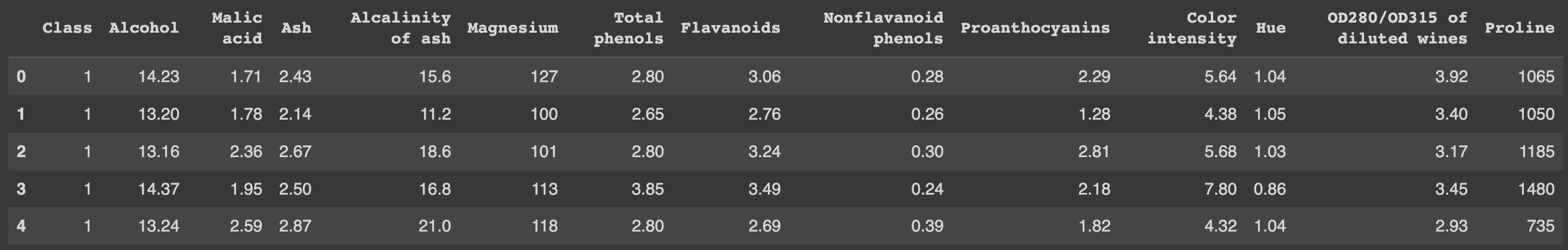
First of all we are going to import the dataset with some basic libraries, and see if it was loaded correctly, also give an overview of the data with their attributes.

import numpy as np
import pandas as pd
import matplotlib.pyplot as plt
import seaborn as sns

df = pd.read_csv("wine.csv")

X = df.drop('Class', axis=1)  
y = df['Class'] 

df.head()

Click the image to watch it fullscreen.

Data Analysis

Once we already verify that all things all correct, we can jump on some characteristics that this dataset have.

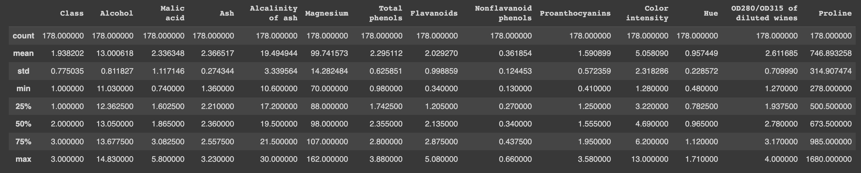
#Statistical Analysis:
df.describe()

#Datatype Information:
df.info()

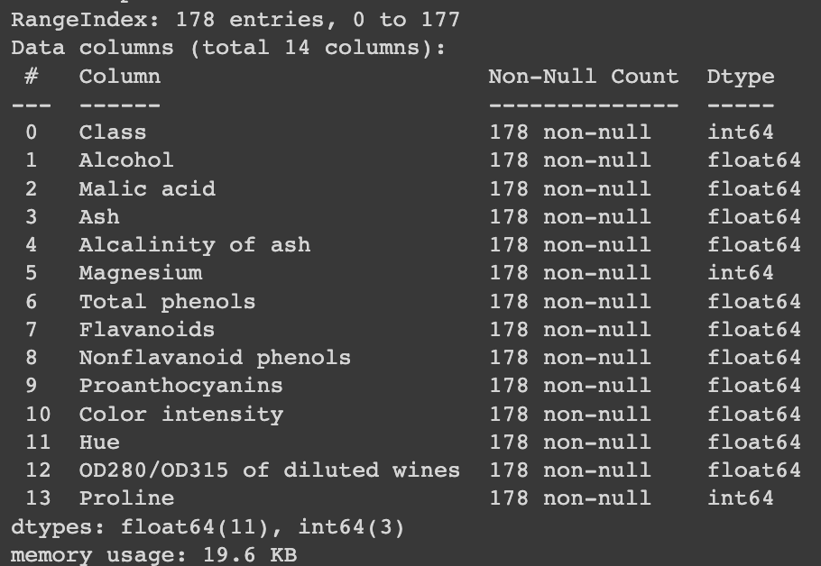
From this tables we can extract some useful information. Firstly, that this dataset hasn’t have any missing values, so that makes the job easier. Additionally, we can see that the ranges of the different attributes have a lot of variances between each other, this might be a problem when we train this set because features such as “Magnesium” will have a lot of weight compared to “Nonflavanoid phenols” or “Hue”. We can solve this problem by using a type of transformation, to know which transformation, we must analyze the distribution of the data.

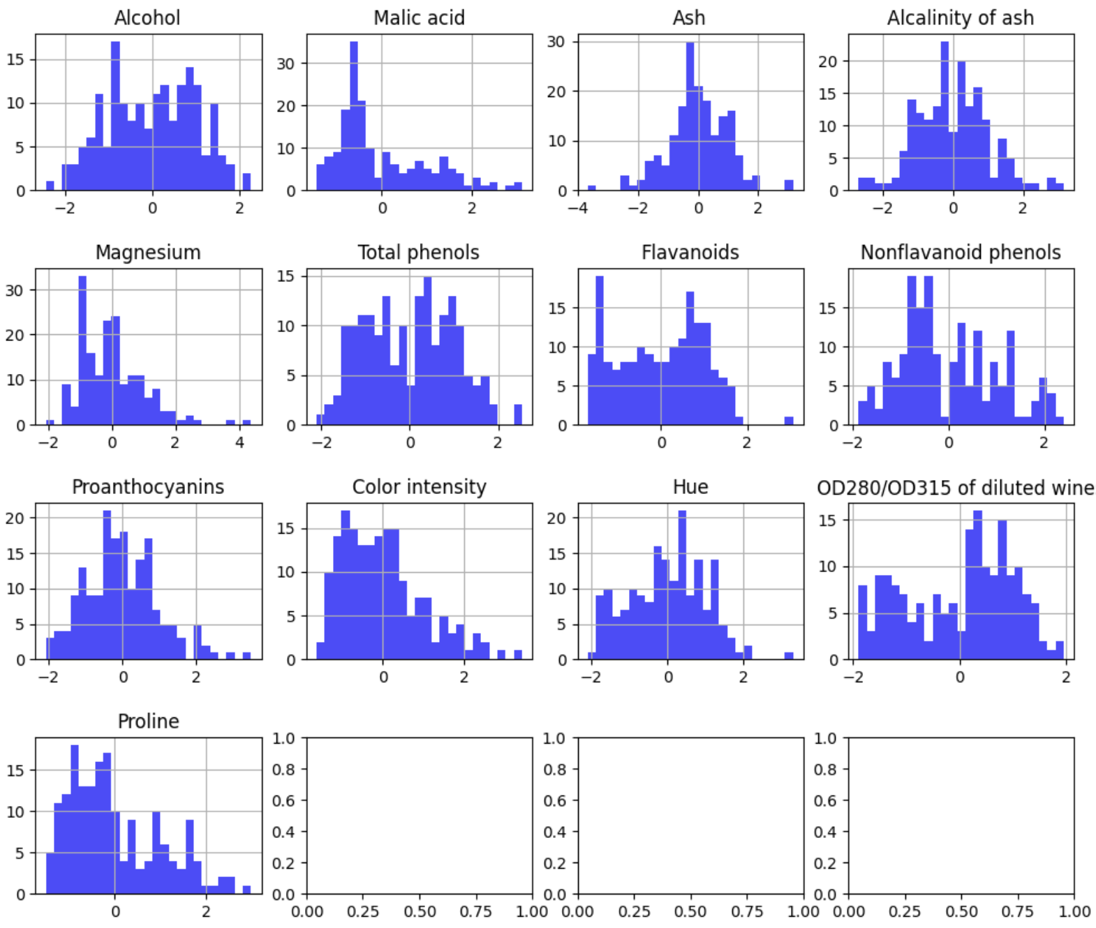
features = df.drop('Class', axis=1)

fig, axes = plt.subplots(nrows=4, ncols=4, figsize=(12, 10))
fig.subplots_adjust(hspace=0.5)

for i, col in enumerate(features.columns):
    ax = axes[i // 4, i % 4]
    features[col].hist(bins=25, color='blue', alpha=0.7, ax=ax)
    ax.set_title(col)

plt.show()

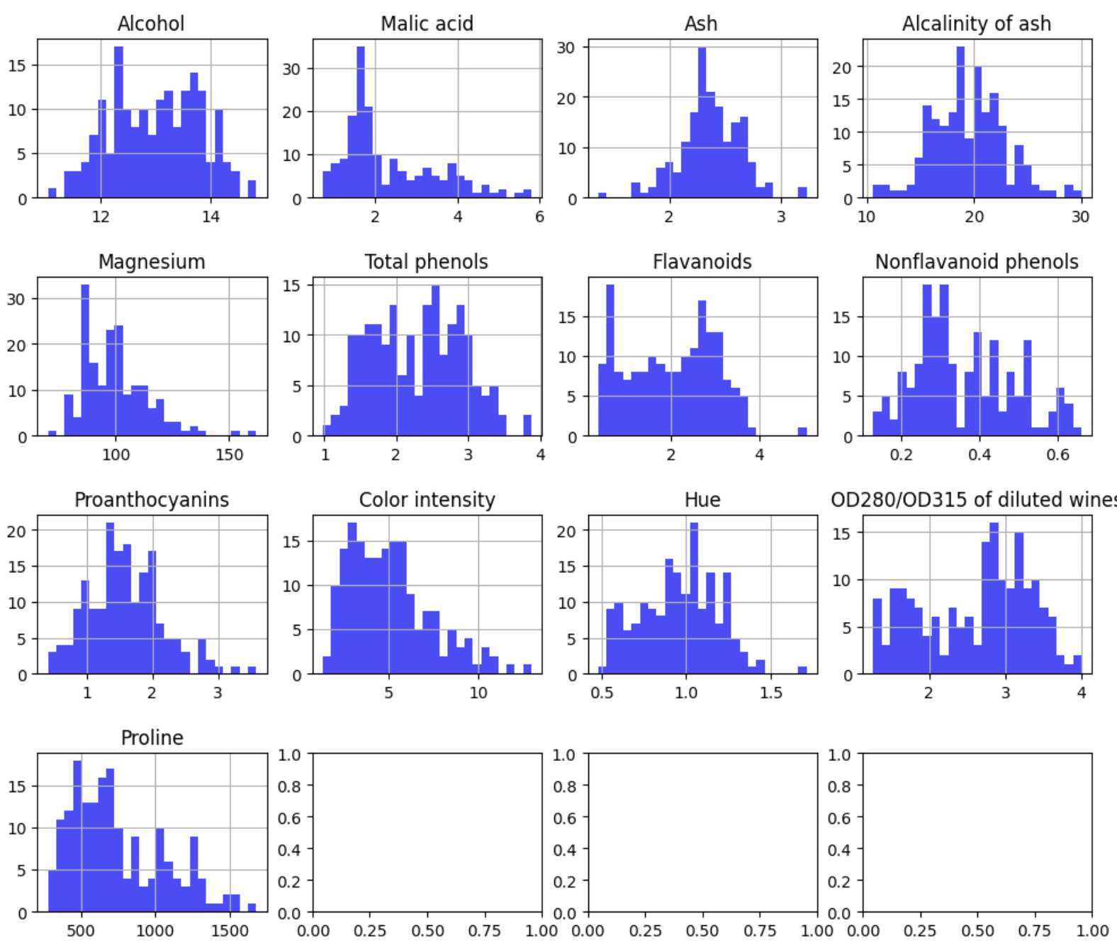
Looking at these histograms we can we that most of the features have a Gaussian distribution, therefore the best option is the z-transformation. Additionally here we can see that it is possible the existence of outliers, something that we are going to analyze further on.

#Applying 

scaler = StandardScaler()
X_normalized = scaler.fit_transform(features)

X_normalized_df = pd.DataFrame(X_normalized, columns=features.columns)

fig, axes = plt.subplots(nrows=4, ncols=4, figsize=(12, 10))
fig.subplots_adjust(hspace=0.5)

for i, col in enumerate(X_normalized_df.columns):
    ax = axes[i // 4, i % 4]
    X_normalized_df[col].hist(bins=25, color='blue', alpha=0.7, ax=ax)
    ax.set_title(col)

plt.show()

Now that the data have mean of 0 and standard deviation of 1, we will have much better results!

Outliers

Now it’s time to analyze if there are any outliers, for that we are going to use some boxplot to view it graphically.

#lets see whether our data has outliers or not:

# create box plots
fig, ax = plt.subplots(ncols=5, nrows=3, figsize=(20,10))
index = 0
ax = ax.flatten()

for col, value in X_normalized_df.items():
    sns.boxplot(y=col, data=X_normalized_df, color='b', ax=ax[index])
    index += 1
plt.tight_layout(pad=0.5, w_pad=0.7, h_pad=5.0)

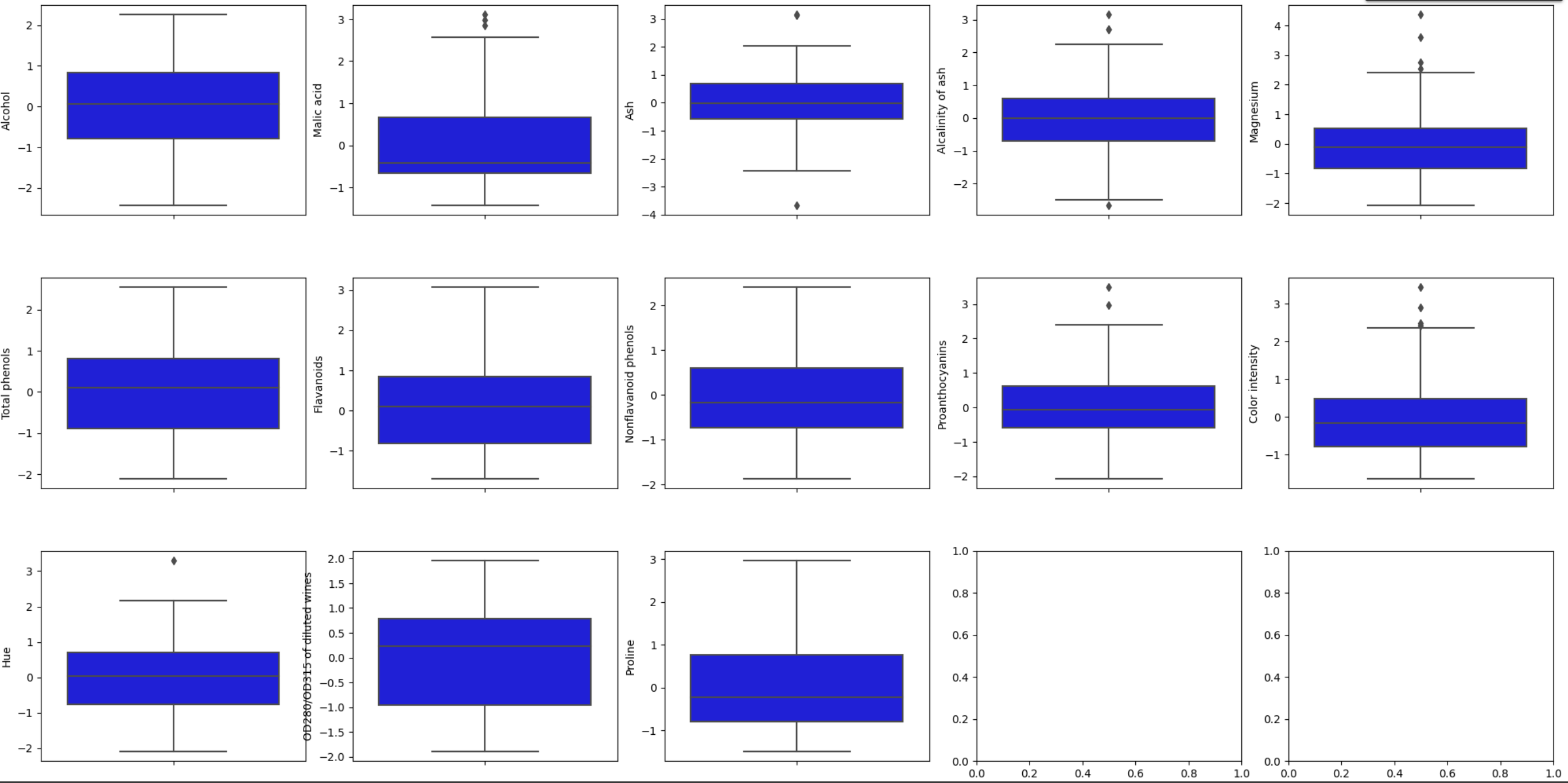
Here we can see that there are some outliers in: “Malid Acid”, “Ash”, “Alcalinity of ash”, between others. But we have to be careful at moment of choosing a threshold for the outliers, if we choose a value for the threshold to low (like 1 or 1.5) we can delete a big amount of data, considering that we only have 178 rows, we have to aim for a higher threshold and remove those outliers that are further away from the majority of the data or have significantly higher values. The threshold chosen was 2.7 with the following results.

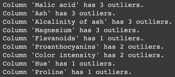
def detect_outliers(column, threshold=2.7):
    mean = np.mean(column)
    std_deviation = np.std(column)
    outliers = (column - mean).abs() > threshold * std_deviation
    return outliers

columns_with_outliers = []

for column in X_normalized_df.columns:
    outliers = detect_outliers(X_normalized_df[column])
    if outliers.any():
        columns_with_outliers.append(column)
        print(f"Column '{column}' has {outliers.sum()} outliers.")

#data normalized and without outliers
sns.pairplot(df_sin_outliers)

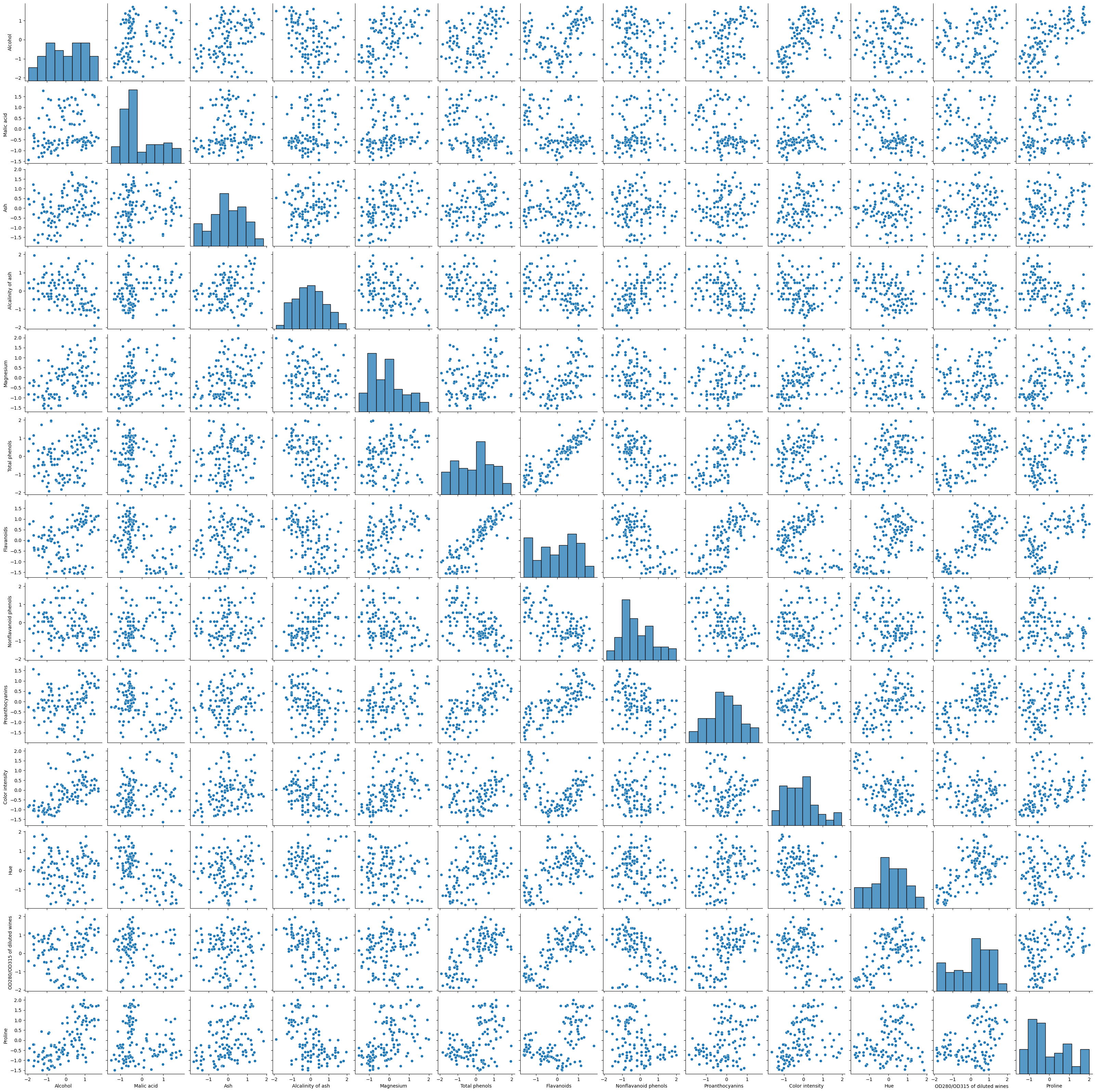
Now that the data is normalized and the outliers were deleted, we can focus more on the correlation of attributes.

Correlated Attributes

Attributes that are correlated could make a big difference in terms of accuracy and performance for a lot of models, that’s why we are going to focus in this topic and specifically in this correlated matrix.

plt.figure(figsize=(15,10))
sns.heatmap(df.corr(), annot=True, fmt='.2f', linewidths=2)

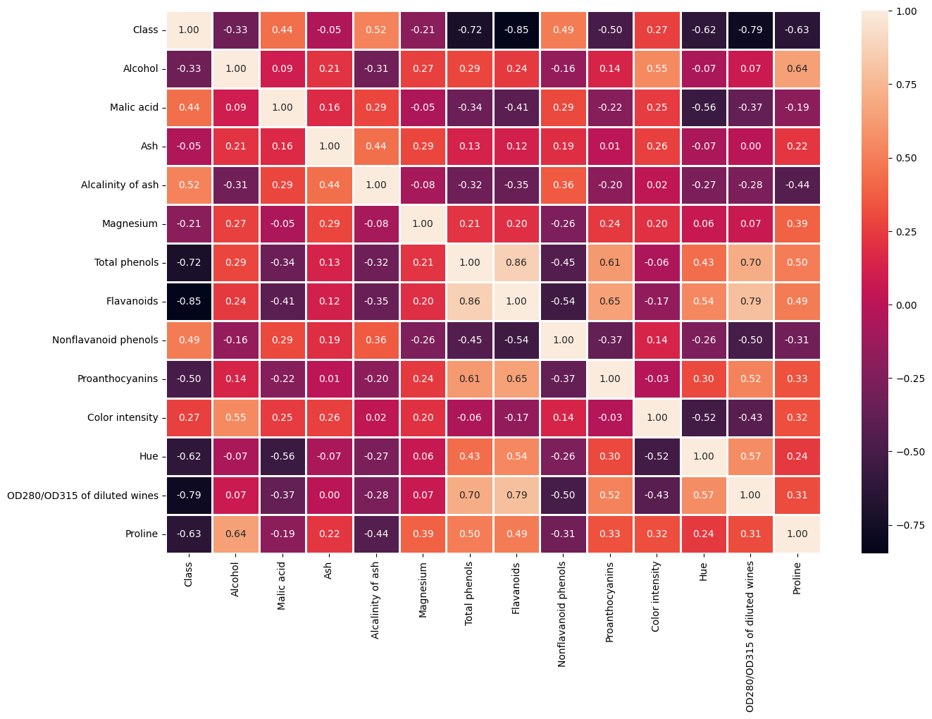
We have a lot of things to analyze here. Firstly, focusing on the attribute ‘Ash,’ we can see that it has a weight of -0.05 on the label, due to this we can delete this attribute since its almost useless for the label and it will improve the performance. Secondly, if we focus on weights of the label, we can clearly see that there are 3 attributes that are ±0.70 or more, which represent a lot of the variance of the label. Those are “Total phenols”, “Flavanoids” and “OD280…”, the thing with these attributes is that there are strongly correlated with each other (±0.70), this could be a problem because perhaps there are describing the same thing and is not needed 3 attributes. After thinking for a while, I came up with some solutions.

• My first possibility was trying to merge “Total Phenols” and “Flavanoids”

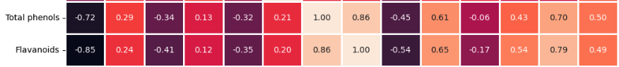
As we can see not only are they correlated with each other, but also the correlation values of the other variables are very similar. For example, taking “Alcohol” as an example, “Total Phenols” has a correlation of 0.29 while “Flavanoids” has a correlation of 0.24. This trend is with all attributes. After making some testing merging this two (and the third later) the results show me that isn’t a good idea because it gave less accuracy that not doing anything with this problem (ignore it). That’s why I jumped for my second and third possibility.

• Using a type of dimension reduction.

The first one that I tried was PCA, since I have already made some work on it and the results were successful. I used the dataset without outliers and with the normalize data, but even that wasn’t useful, it was an improve compared to my first possibility, but it wasn’t enough. Perhaps because PCA deleted some useful information. (tested later on the document)

That’s why I decide using LDA (Linear Discriminant Analysis), one of the main characteristic of LDA is that it maximize separation between different classes in the data, which makes it a supervised technique and its goal is to find the directions in which classes are most separable. The results of using LDA were clearly much better than the other possibilities.

Model Prediction

Now it’s time to test with different models, with PCA, with LDA and without anything.

Random Forest

The first one its Random Forest, which it’s an ensemble algorithm that combines multiple decision trees to improve accuracy and reduce overfitting. It’s a solid choice for many applications due to its ability to handle both categorical and numerical features, as well as dealing with imbalanced data.

clf = RandomForestClassifier(random_state=42)
y = y[df_sin_outliers.index]

# Perform cross-validation and get accuracy scores without outliers
scores = cross_val_score(clf, df_sin_outliers, y, cv=5)
mean_accuracy = scores.mean()
print("Mean Accuracy with Random Forest after Removing Outliers:", mean_accuracy)

# PCA Dimensionality Reduction
pca = PCA(n_components=2)
X_pca = pca.fit_transform(df_sin_outliers)

# Initialize Random Forest Classifier for PCA data
clfPCA = RandomForestClassifier(random_state=42)
scoresPCA = cross_val_score(clfPCA, X_pca, y, cv=5)

mean_accuracyPCA = scoresPCA.mean()
print("Mean Accuracy with Random Forest after PCA Dimensionality Reduction:", mean_accuracyPCA)

# LDA Dimensionality Reduction
lda = LinearDiscriminantAnalysis(n_components=2)
X_lda = lda.fit_transform(df_sin_outliers, y)

# Initialize Random Forest Classifier for LDA data
clf_rf = RandomForestClassifier(random_state=42)
scores_rf_lda = cross_val_score(clf_rf, X_lda, y, cv=5)

mean_accuracy_rf_lda = scores_rf_lda.mean()
print("Mean Accuracy with Random Forest after LDA Dimensionality Reduction:", mean_accuracy_rf_lda)

SVC

The next one its SVC (Support Vector Classification). It is a versatile machine learning algorithm used for solving binary classification problems. Its primary objective is to find an optimal decision boundary that effectively separates data points belonging to different classes while maximizing the margin between them. SVC is known for its ability to handle non-linear data patterns and is widely employed in various domains, making it a fundamental tool in the field of machine learning and data science.

# Initialize Support Vector Classifier (SVC)
clf_svc = SVC(random_state=42)
y = y[df_sin_outliers.index]

# Perform cross-validation and get accuracy scores without outliers
scores_svc = cross_val_score(clf_svc, df_sin_outliers, y, cv=5)
mean_accuracy_svc = scores_svc.mean()
print("Mean Accuracy with SVC after Removing Outliers:", mean_accuracy_svc)

# PCA Dimensionality Reduction
pca = PCA(n_components=2)
X_pca = pca.fit_transform(df_sin_outliers)

# Initialize SVC Classifier for PCA data
clf_svc_pca = SVC(random_state=42)
scores_svc_pca = cross_val_score(clf_svc_pca, X_pca, y, cv=5)

mean_accuracy_svc_pca = scores_svc_pca.mean()
print("Mean Accuracy with SVC after PCA Dimensionality Reduction:", mean_accuracy_svc_pca)

# LDA Dimensionality Reduction
lda = LinearDiscriminantAnalysis(n_components=2)
X_lda = lda.fit_transform(df_sin_outliers, y)

# Initialize SVC Classifier for LDA data
clf_svc_lda = SVC(random_state=42)
scores_svc_lda = cross_val_score(clf_svc_lda, X_lda, y, cv=5)

mean_accuracy_svc_lda = scores_svc_lda.mean()
print("Mean Accuracy with SVC after LDA Dimensionality Reduction:", mean_accuracy_svc_lda)

KNN

And lastly, KNN (K-Nearest Neighbors). It works by finding the k closest data points to a given one and making predictions based on their majority class (for classification) or their average (for regression). KNN is simple, doesn’t assume data distributions, and is widely applied in pattern recognition and data analysis.

# Initialize k-Nearest Neighbors (KNN) Classifier
clf_knn = KNeighborsClassifier(n_neighbors=5)
y = y[df_sin_outliers.index]

# Perform cross-validation and get accuracy scores without outliers
scores_knn = cross_val_score(clf_knn, df_sin_outliers, y, cv=5)
mean_accuracy_knn = scores_knn.mean()
print("Mean Accuracy with KNN after Removing Outliers:", mean_accuracy_knn)

# PCA Dimensionality Reduction
pca = PCA(n_components=2)
X_pca = pca.fit_transform(df_sin_outliers)

# Initialize KNN Classifier for PCA data
clf_knn_pca = KNeighborsClassifier(n_neighbors=5)
scores_knn_pca = cross_val_score(clf_knn_pca, X_pca, y, cv=5)

mean_accuracy_knn_pca = scores_knn_pca.mean()
print("Mean Accuracy with KNN after PCA Dimensionality Reduction:", mean_accuracy_knn_pca)

# LDA Dimensionality Reduction
lda = LinearDiscriminantAnalysis(n_components=2)
X_lda = lda.fit_transform(df_sin_outliers, y)

# Initialize KNN Classifier for LDA data
clf_knn_lda = KNeighborsClassifier(n_neighbors=5)
scores_knn_lda = cross_val_score(clf_knn_lda, X_lda, y, cv=5)

mean_accuracy_knn_lda = scores_knn_lda.mean()
print("Mean Accuracy with KNN after LDA Dimensionality Reduction:", mean_accuracy_knn_lda)

Conclusion

This document presents a comprehensive analysis of the Wine dataset, commencing with a thorough examination of the data and addressing the intricacies of correlated attributes. Throughout our exploration, we have evaluated various strategies, ultimately discerning that KNN and SVC emerged as the top-performing models. However, we must approach these results with caution. It’s noteworthy that LDA didn’t miss any predictions, particularly in models like SVC. This could be an indication of an overfitting model. While it might be acceptable in this instance due to the dataset’s size and features, in the future, to sustain the model’s performance, retraining might be necessary to ensure more precise and accurate results. But we observed that dimensionality reduction using LDA yielded superior results when compared to alternative techniques.